All about the Geo Time Series Model

Geo Time Series (GTS) are at the core of the Warp 10 platform. Only GTSs can be stored in the Warp 10 storage engine, and they are first-class citizens in both FLoWS and WarpScript. That's why there are so many WarpLib functions for their manipulation and so many blog posts making mention of GTS!

Therefore, understanding the GTS model is the first step in mastering the Warp 10 platform. Fortunately, this model is quite simple, yet powerful, and this post will go through most of its aspects.

What are Geo Time Series?

Geo Time Series is a model to represent time series data with an optional location information for each point.

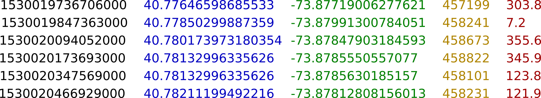
If you prefer an example, imagine an air pollution sensor on a bus coupled to a GPS. This sensor takes the reading of ozone levels from time to time while the bus is moving. The sequence of readings, each one composed of a timestamp, a latitude, a longitude, an elevation, and an ozone level, form a series.

As we will index time, we call them time series and as we will not only have the value of the sensor but also its geo-location, we call them Geo Time Series.

GTS are indexed on time, so you can easily select a time range and get the associated values and locations. You can also index locations, but this is not done by default. The index on time is used when getting the data from a storage (LevelDB, HBase, memory, HFile, S3, etc.) but also when manipulating the GTS, most notably with frameworks.

Value as a Function of Space and Time

You should ask yourself: why grouping locations and values in a single model? It is indeed possible to have a time series of latitudes, one of longitudes, one of elevations, and one of values. The advantage of the GTS model is threefold.

First, this contextualizes the measured value. If we keep the same air pollution example as above, it is obvious that the level of ozone is highly dependent on the time, but also the location of the sensor. Mathematically, we can see the recordings as samples of a function f(time, location)=ozone, which are all, conveniently, in the same model.

Second, this makes the data more compact. Splitting the data in several time series would require the duplication of the timestamps. If you multiply that by billions or trillions of recordings, the gain can be important. Be careful though, you can't generalize that to any value. For instance, if we had a tabular model, factorizing the timestamp for several sensors, would the sensors have very different sampling frequencies, say 1Hz and 100Hz, this would lead to almost empty tables. Even if some solution to avoid losing space can be found, the manipulation of such a table wouldn't be convenient.

Third and last, this makes analysis much easier. Having all this information in the same model is much more convenient than having to combine several structures. You can easily analyze the influence of altitude on pollution or restrict your analysis to a specific area.

Geo Time Series are a Superset of Time Series

For still sensors, it is obviously not a good idea to store their positions for each value. Good news, the latitude/longitude couple and the elevation are both optional! This case is well handled by Warp 10 and storing GTS without location and loading them into memory does not take any space to represent "missing" locations. There is no downside to using Geo Time Series without locations.

In that sense, Geo Time Series are a superset of time series because GTS can both associate timestamps to represent values or values/locations couples. Very often, a good GTS model mixes the two types of GTS. For instance, when you have a really high-frequency sensor on a slow-moving object, like fiber optics in a yacht, storing the location is a bad idea because the location will be pretty much the same for thousands of consecutive records. If you need to combine those high-frequency sensors with location data during analysis, this is indeed possible.

Values in Geo Time Series

Until now, we focused on space and time aspect of the GTS, but it's time to focus on the values. GTS can store 4 main types of values: Booleans, Longs, Doubles, and Strings. With only these types we aim at covering any use-case.

Booleans are the simplest values a GTS can store: true or false, that's it. Even if very simple, they are extremely useful: is an alert triggered? Are landing gears on the ground? They also have a very small disk and memory footprint which makes them perfect to optimize some computations.

Next, are probably the most common types: numerical GTS. A lot of sensors give floating-point or integer numbers, like temperature, squawk codes, number of writes, etc. They take more space than boolean GTS, still, the storage is optimized for both Longs and Doubles.

Last are Strings, which is the most versatile type but is not optimized as other types. String values can store annotations or log messages for instance. It can also be used to store more complex structures like JSON or base64 Strings which make possible the serialization and deserialization of Objects stored in GTS.

Going further, we even allowed the storage of binary values in GTS, which are represented as GTS of ISO8859-1-encoded Strings. Going even further, we allowed the storage of encoded GTS as binary values in GTS, we call that multi-values. This makes possible very complex data models that both have great performance and are easy to use.

Organizing Geo Time Series

Name your Geo Time Series

Now that we defined precisely the content of GTS, it's time to see how we identify a single GTS or a specific subset of GTS. Every GTS is uniquely identified by a classname and optional key-value pairs called labels. This is exactly the same principle as Prometheus with its metric name and labels and OpenTSDB with its metric name and tags, not a surprise since all those tools were inspired by the model used in Google's borgmon. It is very important to understand that the classname and labels form a unique identifier. Change anything, a label value for instance, and you're referring to another GTS.

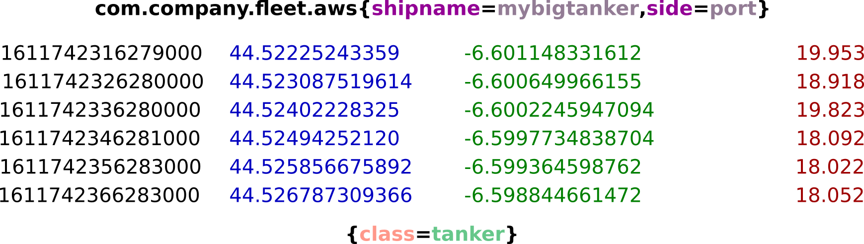
Let's take an example. Imagine you have fitted 2 wind speed sensors on a tanker. The classname usually defines the measured value. In our case, for the two GTS, the classname would be com.company.fleet.aws as AWS means Apparent Wind Speed. Next, we use the labels to define precisely the sensor. We can use almost as many labels as we want, but two will be sufficient: shipname and side. Finally, we select values for labels, mybigtanker will be associated to shipname and one sensor will have the port associated to side while the other have starboard.

You can see how com.company.fleet.aws{shipname=mybigtanker,side=port} will uniquely identify a single sensor. You must be very careful not to add any label which could change in the lifetime of the metric. In this case, adding something like the brand of the sensor or the destination of the tanker is probably a bad idea because the sensor could be replaced, and the destination is bound to change. GTS are already indexed on time, so there is little advantage of adding a time-dependent label.

Select your Geo Time Series

The way GTS are named easily allows the definition of GTS sets using what we call selectors. You want all AWS GTS on the ship? Query com.company.fleet.aws{shipname=mybigtanker}, unspecified labels can take any value. You want all GTS on your tanker? Query ~com.company.fleet.*{shipname=mybigtanker}, ~ means that the following classname is a regular expression. You can also use the same logic on label values to select several ships with com.company.fleet.aws{shipname~my(big|small)tanker}.

Would you need to add extra information to a GTS which is not essential to its identification? You can add attributes. Attributes are also key-value pairs but are mutable. You could add the {class=tanker} attribute to your GTS which would let you easily select all tankers the same way you use labels in selectors.

Manipulating Geo Time Series

It would be too long to list all the possible manipulation that can be done on GTS, but we will give you some pointers to useful resources. As we are manipulating time series, time is of utmost importance in almost all GTS-related functions. For instance, the MAP framework lets you apply a function on a sliding window over the GTS. REDUCE combines points from different GTS sharing the same timestamp, etc.

Those two functions are part of the frameworks which are almost always at the very core of every single script you will write. These are very powerful and versatile functionalities which can, for instance, synchronize timestamps between GTS or makes timestamps evenly spaced from irregular data.

Apart from frameworks, other more specialized functions make the analysis of time series data a lot easier. Some functions allow the splitting of GTS according to different parameters: time or distance between consecutive points or more complex stop detection. It is also possible to detect anomalies in GTS using different algorithms.

All those functions avoid the need of rewriting complex code each time you need to design a script for the analysis of time series. This saves you development time and lets you focus on the logic of your analysis.

Bending Geo Time Series to your Will

This post wouldn't be complete if we didn't talk about how to corrupt this GTS model. A word of warning, this section is about very advanced GTS modeling and manipulation.

First, the locations in a GTS are encoded as 64-bit HHCodes. So, to put it bluntly, a GTS is a sequence of recordings, each composed of 1 Long, 2 optional Longs, and a Boolean, a Long, a Double, or a String. You normally use the 3 Longs to represent the timestamp, the location HHCode, and the elevation, but can in fact represent anything.

If you want to store a GTS, timestamps must be unique in a GTS. You can store a unique identifier in timestamps, for instance, a MMSI identifying a single ship, a OSM way ID, or even a HHCode. This allows you to retrieve rapidly the information you need without needing an additional database to store that kind of information.

If you need your GTS to store 3 Longs per datapoint, you can store them in the location, elevation, and value. By default, the location Long is interpreted as a 64-bit HHCode and converted as latitude/longitude. You can easily retrieve the Long representation with the ->GTSHHCODELONG function. Be careful, the HHCode 91480763316633925 is reserved and means "no location" so you should not store that in the location.

Takeaways

Geo Time Series is a versatile model to represent time series data, well-adapted to data coming from sensors and metrics from a wide range of domains. Geo Time Series can optionally store a location and elevation for each point but there is no downside of using Geo Time Series without locations.

They can store Booleans, Longs, Doubles, and Strings which offers both performance and compatibility with almost any kind of data. To query Geo Time Series, they are uniquely identified by a classname and optional key-value pairs called labels. This allows the selection of a unique series or a group of them to combine and analyze them.

Finally, WarpLib functions offers a wide range of functionalities to manipulate Geo Time Series. The aim of these functions is to save you development time and let you focus on the logic of your analysis.

Fabien Tencé

WarpScript™ Doctor