In this blog post, we review the essential frameworks available in WarpScript. They simplify greatly usual time series processing.

When working with time series, it is worth noting that some pre-processing operations occur frequently.
For example, you would often need to:
- Sub sample your data
- Align the ticks
- Evenly space out the ticks
- Apply a function on each tick of your time series
- Handle missing values
- Apply operations between various time series
- Apply a function on values caught in a sliding window for each step
- Etc. (this list is not exhaustive)
Luckily, one of the key strengths of WarpScript is that it has been thought for time series analysis so that frequent operations are easy to implement in just a few lines of code.
| Learn more about WarpScript. |
At SenX, we identified a few frameworks that allow performing all the usual time series processing, and of course, these frameworks are built into WarpScript. Note that we call framework a WarpScript function that has a function among its arguments.
In this article, we present the essential frameworks. If you consider yourself a novice in time series, we believe that after you understand them, you will realize that it is a lot easier than you thought.
We will illustrate our discussion with examples on a small dataset of hourly temperatures measured in US cities. You can get the data on this link. Remember that if you want, you can push them on the free Warp 10 Sandbox and get your hands on them in no time.
FILTER
The first framework, FILTER, is the simplest one. From a list of GTS (abbreviation for Geo Time Series), it selects those matching some criteria. These criteria are defined by a function called a filter.
For example, the WarpScript below fetches some data, then keep the GTS according to the value of the "city" label:
// Make sure we can fetch enough datapoints
'<insert-your-token-here>' 'token' STORE
$token AUTHENTICATE
2000000 LIMIT

// Fetch dataset
[ $token 'temperature' {} NOW NOW ] FETCH
// Remove unused meta information (for viz)
{ '.app' '' '.uuid' '' } RELABEL 'data' STORE

// Filter to get our wanted GTS
[ $data [] { 'city' 'San Francisco' } filter.bylabels ] FILTER
0 GET 'sf_gts' STORE
Note that the second argument of FILTER is left here as an empty list and is rarely used. We will talk about it later.
Indeed, we could have done directly [ $token 'temperature' { 'city' 'San Francisco' } NOW NOW ] FETCH to obtain San Francisco's temperature measurements in fewer lines. But fetching only once and using FILTER is better if we need both the whole $data and the particular $sf_gts in the remaining of the WarpScript.
BUCKETIZE
In the numbered list from the introduction, the BUCKETIZE framework allows you to solve in one-line bullets 1 to 3. Intuitively, it creates "buckets of time". The buckets are all the same size, contiguous and non-overlapping. In each bucket, data are aggregated into a single datapoint using a function called a bucketizer. The timestamp associated with each bucket is its most recent one.
As a consequence, ticks of resulting time series are evenly spaced out, and if you apply BUCKETIZE on a list of multiple input time series, their ticks will be aligned (unless you did not use a common value for the last bucket parameter). It can also be used for sub-sampling.
For example, in the following WarpScript, we bucketize the hourly input data, into daily buckets:
// Bucketize
[ $sf_gts bucketizer.mean 0 1 d 0 ] BUCKETIZE
0 GET
'bucketize result' RENAME
'sf_bucketized' STORE

// Leave input and output on the stack to plot them
$sf_gts
$sf_bucketized
In WarpStudio editor, we obtain the figure below by zooming in the Dataviz tab and choosing a step plot:
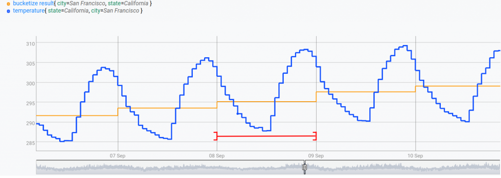
The red interval delimits values that are considered in the bucket to compute the value on sept. 9th.
MAP
The MAP framework answers bullets 4 and 5 from the list above. For each of its input time series, it computes a new value at each tick that depends on neighboring values defined by a sliding window. The size of the sliding window is the same at each tick and is determined by arguments passed to MAP. Sliding windows can be defined in a number of ticks or time units. The function that is used to compute the new value at each tick is called a mapper.
For example, you can compute the moving mean in the last day with MAP:
// Map
[ $sf_gts mapper.mean 1 d -1 * 0 0 ] MAP
0 GET
'map result' RENAME
'sf_mapped' STORE

// Leave input and output on the stack to plot them
CLEAR
$sf_gts
$sf_mapped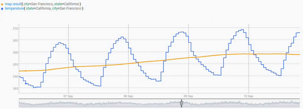
Contrary to BUCKETIZE, we obtain one value per value present in the input GTS.
| You need only 7 lines of WarpScript to filter out data when there are timestamp irregularities |
REDUCE
Even though BUCKETIZE and MAP can be applied on a list of GTS, they operate on each one independently of the others.
On the other hand, REDUCE reduces groups of GTS into single ones. This reduction is done using functions that are called reducer. The reducer is called on each tick such that there is at least one input GTS that has a value at this tick (and if the result of the reducer is null, no value is produced at this tick for the resulting GTS). This framework can handle bullets 6 and 7 from the list above.
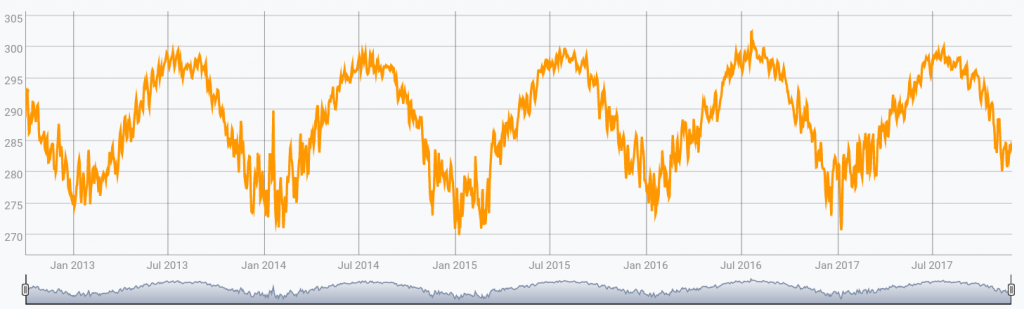
For example, let's consider the following WarpScript:
[ $data bucketizer.mean 0 1 d 0 ] BUCKETIZE
[ SWAP [] reducer.mean.exclude-nulls ] REDUCE
This WarpScript takes all input GTS, and produces a GTS which values are the means of the input GTS at each tick.
Note that it is possible that some input GTS has no value at a given tick. This is why we use reducer.mean.exclude-nulls since it produces a value on these ticks whereas reducer.mean does not. Also, note that it is good practice to use BUCKETIZE before a REDUCE in order to align the ticks correctly.
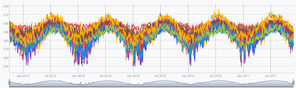
Given this list of input GTS:
The WarpScript above produces the following output:
Grouping by labels
The second argument of REDUCE and FILTER is a list of label keys. This argument is often left as an empty list, as done in the previous examples. However, it can also be used to group the input GTS by the values on these labels.
For example, let us modify a bit the previous WarpScript:
[ $data bucketizer.mean 0 1 d 0 ] BUCKETIZE
[ SWAP [ 'state' ] reducer.mean.exclude-nulls ] REDUCE
The second argument of REDUCE is a list that contains the label key "state". So, REDUCE will first group the input GTS by state. Then it will reduce each group. The output of REDUCE is then a list containing one GTS per state.
We obtain the following output:
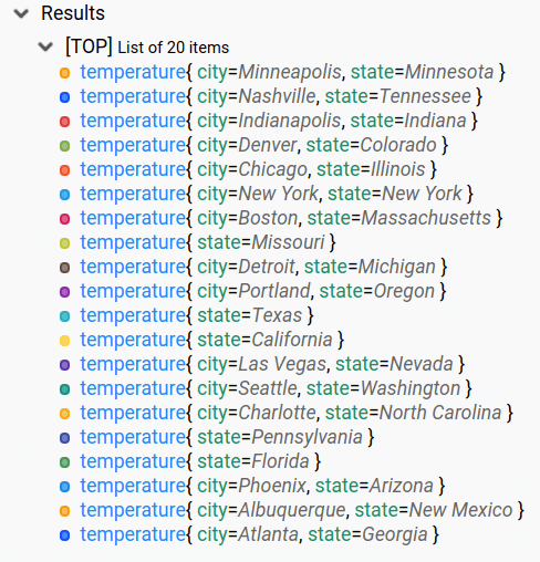
Note that in this output list, for states that had data for only one city, the corresponding GTS kept the city label. On the other hand, state that had data for more than one city had their GTS regrouped and reduced.
Conclusion
In this article, we presented the essential frameworks, namely FILTER, BUCKETIZE, MAP and REDUCE. These frameworks allow doing in a few lines of code the most usual operations (and more!).
Each of these frameworks uses a function, respectively, a filter, a bucketizer, a mapper, or a reducer. In a future blog post, we will talk about how to define custom versions of these functions, if those available in the WarpScript library do not suffice your needs!
Read more
Matrix Profile of a Time Series to discover Patterns
Protecting your Macros and Functions with Capabilities
Working with GEOSHAPEs

Machine Learning Engineer