Working with GEOSHAPEs

Warp 10 is unique in the time series platform landscape because of the way it handles location data. The core data structure of Warp 10 is called Geo Time Series and considers time, value, and location as first-class citizens. The Warp 10 Analytics Engine makes it easy to manipulate location data using the numerous geo-related functions present in WarpLib.

Among the possibilities offered by Warp 10 is everything related to geographical areas with applications such as geofencing, knowing when a locating is within a given zone, and geo calls, i.e. determining which zones a given trajectory intersects. Both of these applications can be implemented using dedicated solutions such as Elasticsearch or PostGIS. But this would render your infrastructure more complex. In this article, we will show you how you can do all those operations right within Warp 10.

HHCodes and GEOSHAPEs

As already exposed in a previous article, Warp 10 uses a grid mechanism called HHCodes to represent location. This grid system allows the representation of locations down to a precision below the centimeter, good enough for 99.999999% applications out there. So each location on earth has an associated HHCode, the one for that red paper clip on the left of my computer is b570f9721ebca2df.

HHCodes are 64 bits numbers, but by considering only a subset of those bits you end up with cells of increasing sizes. Try to run the following code in WarpStudio. You will see nested cells which represent the location of that red paper clip at different resolutions.

'T3JUXkV.........Ht3DttyiyEeJQccqY53CNrY25C3kGYPBJFpYSBBNgq5BpI25QWYYC7ll5wOs2LEwWY7.gzECIcR....L6W3.'
GEOUNPACK
'zone' STORE

{
  'data' [ $zone T ->GEOJSON JSON-> ]
}

The cryptic string T3J.... is a packed Geo Shape, this is a packed list of HHCode cells. A HHCode cell is a 64 bits number whose lower 60 bits are a HHCode shifted right 4 bits and the upper 4 bits are a resolution, from 1 to 15, specifying how many bits of the 60 should be considered: 4 bits for resolution 1 to 60 bits for resolution 15. A collection of HHCode cells, therefore, represent a geographic zone, in Warp 10 this is called a GEOSHAPE.

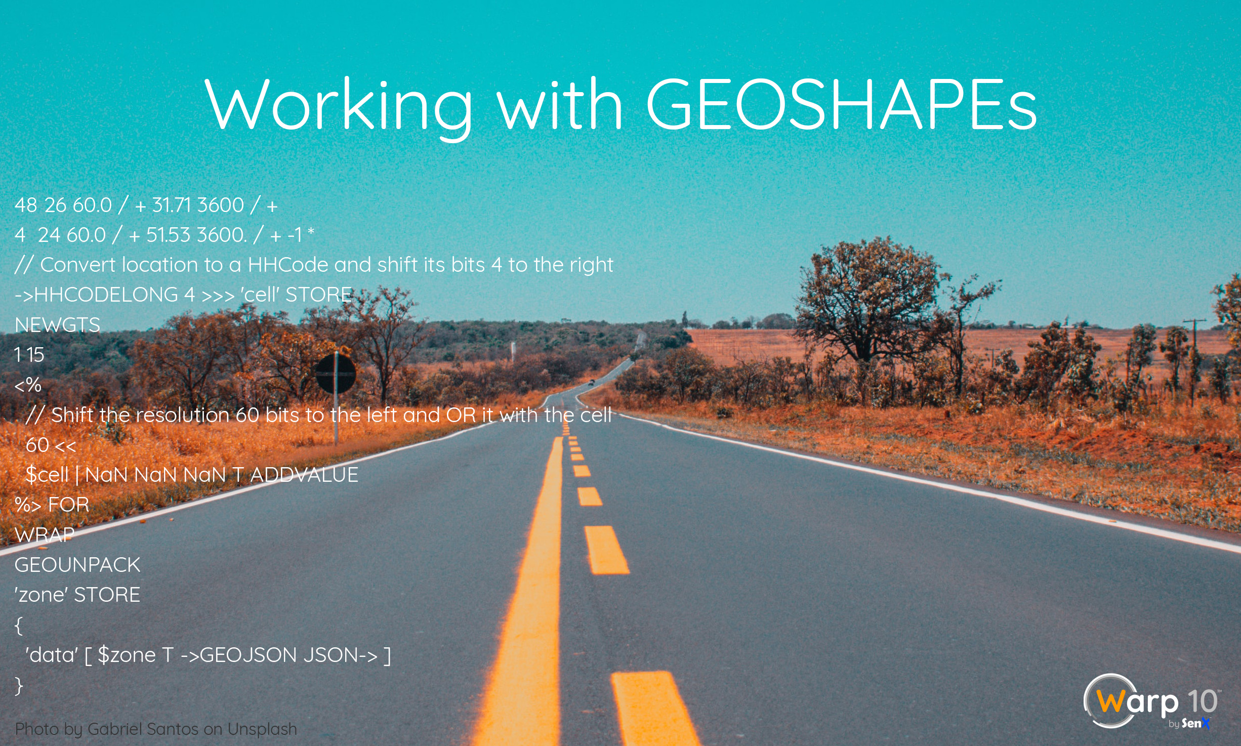
The magic behind GEOSHAPEs is that their packed form is actually a wrapped Geo Time Series where timestamps are HHCode cells and values are boolean true. So you may create a GEOSHAPE using NEWGTS, ADDVALUE , WRAP and GEOUNPACK. The following code does just that for the GEOSHAPE above:

48 26 60.0 / + 31.71 3600 / +4  24 60.0 / + 51.53 3600. / + -1 *

// Convert location to a HHCode and shift its bits 4 to the right
->HHCODELONG 4 >>> 'cell' STORE

NEWGTS

1 15
<%
  // Shift the resolution 60 bits to the left and OR it with the cell
  60 <<  $cell | NaN NaN NaN T ADDVALUE
%> FOR
WRAP
GEOUNPACK
'zone' STORE

{
  'data' [ $zone T ->GEOJSON JSON-> ]
}

Creating GEOSHAPEs from descriptions

As we have just seen, you can create GEOSHAPEs by specifying their cells manually. While this is possible for simple shapes like the example above, it is far too complex for most shapes. This is why WarpLib has functions to create those shapes for you from their descriptions in standard formats. WarpLib currently supports GeoJSON, WKT, and WKB.

You can create GEOSHAPEs from those formats using the functions GEO.WKT, GEO.WKB and GEO.JSON.

Those functions allow you to specify the resolution at which the shapes should be generated. Whether as a percentage of the diagonal of the shape's bounding box, or as an explicit resolution (an even number from 2 to 30, indicating the number of bits to use for latitude and longitude). You can also choose if the generated GEOSHAPE should be inside the described shape or cover it completely.

For some use cases, it might be useful to be able to specify a buffer around a shape or along a line. The GEO.BUFFER function allows you to do just that.

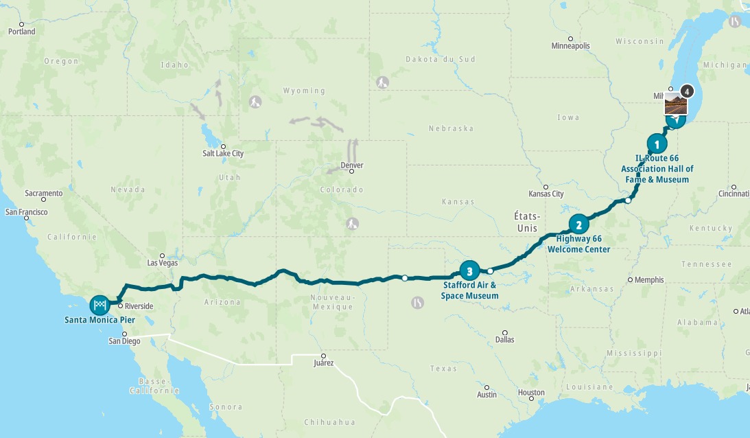
The example US66.mc2 generates a shape covering the historical route US66 by creating a buffer 20 meters on each side of the road. The GeoJSON description of the shape is 3,966,302 bytes (633,699 when gzipped) while the packed GEOSHAPE is only 165,426 bytes (124,069 raw bytes), that is a reduction of 80.5% compared with the compressed GeoJSON.

Combining GEOSHAPEs

The nice thing about GEOSHAPEs is that they can be manipulated like sets, creating new GEOSHAPEs which are unions, differences, or intersections of other shapes.

This allows to create complex shapes which can later be used for performing geofencing or calls operations.

For example, you could create a GEOSHAPE which covers all the ports of the Atlantic coast of Europe, or one that covers all cities over a certain size, or all airports with runways above a given length. Those shapes can be used just like the ones that were generated from a GeoJSON or WKT description.
Check the functions GEO.UNION, GEO.INTERSECTION, and GEO.DIFFERENCE.

Performing Geo-Fencing

Geo Fencing is the process which consists in determining the relationship between a location or zone and a set of other zones. The most common type of geofencing is to determine if a point is inside or outside a virtual perimeter.

In Warp 10 the GEO.INTERSECTS function can be used to determine if two GEOSHAPEs intersect, or if a Geo Time Series or a list thereof have points which are included in a given shape.

If you want to determine if a single location is within a given GEOSHAPE, you can simply convert that location's HHCode into a GEOSHAPE with the following code:

48.0 -4.55 [ 'lat' 'lon' ] STORE

// Create a GTS Encode to hold the value
NEWENCODER

// Convert lat/lon to HHCode
$lat $lon ->HHCODELONG

// Create a single cell at resolution 30 (0xF prefix)
4 >>> 0xF000000000000000 | NaN NaN NaN T ADDVALUE
WRAPRAW GEOUNPACK
'pointshape' STORE

With the above example, determining if the point (48.0, -4.55) is in a circle of radius 1000 m centered at (48.0, -4.56) can be done like this:

$pointshape
48.0 -4.56 1000 @senx/geo/circle 0.01 F GEO.WKT
GEO.INTERSECTS

If you wanted to actually obtain the intersection GEOSHAPE, simply use GEO.INTERSECTION instead of GEO.INTERSECTS.

Doing zone calls

Zone calling is an interesting use case which often leads to complex solutions being deployed. The goal of zone calling is to identify geographical zones which were crossed by a trajectory.

The typical concrete example is identifying port calls from ship trajectories to understand where a vessel has gone. Another example is determining which vehicles entered contaminated zones and may be at risk of spreading hazards if they are not stopped.

We have seen countless implementations of zone calling which used the wrong tools and thus led to complex infrastructures and even more complex queries.

In Warp 10, performing zone call is very easy. It is a generalization of the determination of GEOSHAPEs intersections, and it can therefore be performed blazing fast even on very complex shapes.

As an example, we will determine which counties of the US are crossed by the US-66 highway introduced above.

The brute force approach will take as input a map of names to GEOSHAPEs and will compute the intersection of each of the shapes with the shape of Route 66. For each match, the county name will be retained.

A more efficient method consists in first checking the intersection with the states and then checking the intersection with the counties for those states.

Note that in neither of those solutions were the shapes indexed. It is purely using WarpLib and therefore the same approach can be performed at scale in a tool like Spark.

Takeaways

The GEOSHAPE type of Warp 10 allows all sorts of location-based applications to be developed without having to add yet an extra component to your infrastructure. We encourage you to explore all the Geo related functions available in Warp 10 and share on the Warp 10 Lounge what you have built.

Mathias Herberts

Co-Founder & Chief Technology Officer