Working with GEOSHAPEs: code contest results

Following Mathias' article about GEOSHAPES, I wrote a little code contest to practice. Here is the result.

Questions to solve

Given the Route 66 geoshape and the GTS from the datalogger:

• How many kilometers did this car on the Route 66?
• Its fuel consumption approximation is 8 (liters/100 km) × (speed (km/h) / 80) +1. One liter of fuel releases 2392g of CO2. How much CO2 did the car release while driving on the Route 66?

Step 1: explore data

It seems obvious, but I met people that try to manipulate data without having a glance first. This step is very important: look at data interval, extrapolate a rough result from what you can guess. The answer to the first question cannot be 2000 kilometers, for example

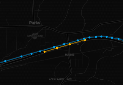
In the contest, I provided a WarpStudio snapshot (a link to a WarpScript). You can click on it, then click on dataviz, and tick the map view.

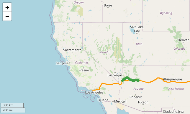
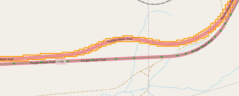
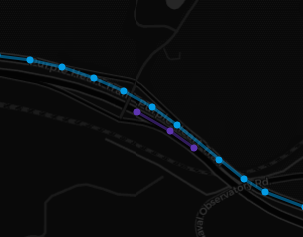
You can see that there is some weird things in the input data: sometimes, the car is on the road, sometimes it is on a parallel road that is not part of the given geoshape. Fine. You have to do with that, do not try to fix input data.

You also see that it is not one-way travel. Where does the drive start? You can SHRINK the input to keep only the first 20 ticks for example:

// Here is the gts of the car datalogger
@senx/dataset/route66_vehicle_gts -100 SHRINK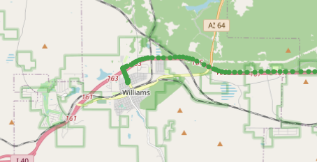

What is the frequency of the data? To find out the delta between each tick, you can use mapper.tick and mapper.delta, then convert it to seconds.

// Here is the gts of the car datalogger
@senx/dataset/route66_vehicle_gts
[ SWAP mapper.tick 0 0 0 ] MAP  
[ SWAP mapper.delta 1 0 0 ] MAP // window size: pre = 1   post = 0
[ SWAP 1.0 STU / mapper.mul 0 0 0 ] MAP

In the code, I chain 3 MAP operations:

• replace values by the tick, for each tick
• compute delta between two values (note the window size)
• divide everything by STU (my Warp 10 is configured in a microsecond, so STU returns 1 000 000)

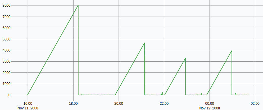
Interesting result: there are some pauses in the GPS record. Around 1 hour of pause sometimes. In my mind, as a WarpScript user, I think "TIMESPLIT will be useful".

If I remove values greater than 100 seconds by adding another mapper :

// Here is the gts of the car datalogger
@senx/dataset/route66_vehicle_gts
[ SWAP mapper.tick 0 0 0 ] MAP
[ SWAP mapper.delta 1 0 0 ] MAP
[ SWAP 1.0 STU / mapper.mul 0 0 0 ] MAP
[ SWAP 100 mapper.lt 0 0 0 ] MAP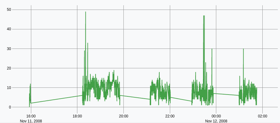

I can see the GPS datalogger records position every 10 seconds or so, with a worst-case of 50 seconds without any data.

So, to sum up:

• The car often leaves the road. The input data are not perfect, the road sometimes splits into different lanes which are not covered by the geoshape. Anyway.
• The system records one data point every 10s, sometimes with a 50s lag.
• The driver took a few naps in the meantime.

Step 2: keep data ON the road

This is a very straightforward task:

• Keep data points that are within the geoshape.
• Split in multiple continuous GTS (continuous = less than 1 minute between two timestamps)
• Keep splits with more than one data point

// Here is the gts of the car datalogger
@senx/dataset/route66_vehicle_gts 'carTrajectory' STORE

// Here is the route 66 geoshape (+/- 20meters)
// For dataviz, convert the shape to geojson, then tick the map button in the dataviz
@senx/dataset/route66_geoshape 'route66SHAPE' STORE // ->GEOJSON JSON->

[ $carTrajectory $route66SHAPE mapper.geo.within 0 0 0 ] MAP // keep datapoints on the route 66
0 GET // get one gts, not a list

{
  'timesplit' 1 m // > 10 minutes between two points
}
MOTIONSPLIT // split in a list of gts
<% SIZE 1 > %> FILTERBY // ignore splits with only one datapoint.
'ListOfSplits' STORE

$ListOfSplits

Here I used MOTIONSPLIT, that can do much more than TIMESPLIT. But TIMESPLIT does the same job here.

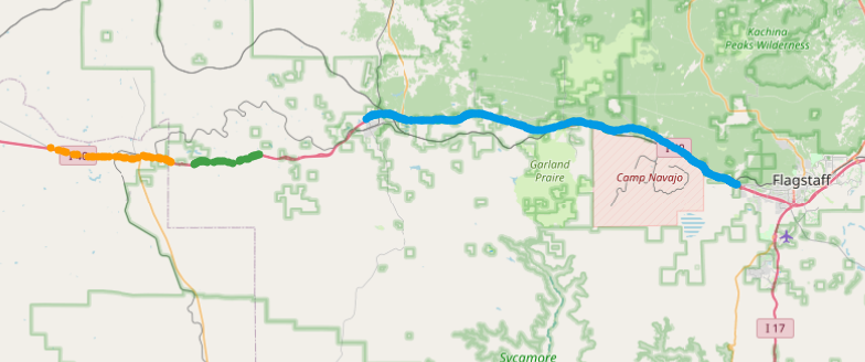
There are three big relevant splits, and a few others that sometimes match the road

The input data is far from perfection, but anyway, I keep all 7 splits.

Step 3: kilometers on the road

Between each data point, we can compute the number of meters. Then sum all these little distances to get the total number of kilometers traveled.

[ $ListOfSplits mapper.hdist 1 0 0 ] MAP // compute distance between each datapoint
'distances' STORE
$distances MERGE // merge splits in one
[ SWAP bucketizer.sum 0 0 1 ] BUCKETIZE // sum all values
'totalDistanceTraveled' RENAME // rename the output gts'

• mapper.hdist does the hard part of the job: compute precisely the number of meters between each data point. The distance between each data point is now the value for every output GTS.
• MERGE take the list of "distance gts" and recreate only one GTS
• bucketizer.sum, used with only one bucket, does the job to sum every value.

The output is a GTS named "totalDistanceTraveled", with only one datapoint that contains the total distance traveled on the Route 66: 79.8 km

Alternative solution: As Nicolas did, you can also use a mapper with a huge window (MAXLONG for pre- and post-parameter):

[ $sectionOnTheRoad mapper.hdist MAXLONG MAXLONG 1 ] MAP
'totalDistancePerSection' STORE
0 $totalDistancePerSection
<% VALUES 0 GET + %> FOREACH

This is perfectly correct and will give you the same result. As a mapper is an aggregator, you can also use it in a BUCKETIZE operation, this will also give you the same result.

// both lines are equivalent
[ $input mapper.hdist MAXLONG MAXLONG 1 ] MAP // map with a huge window
[ $input mapper.hdist 0 0 1 ] BUCKETIZE // bucketize with a single bucket

Step 4: CO2 emissions

The emissions are directly linked to the vehicle speed. So the first step is to compute the instantaneous speed. Thanks to WarpLib, there is already a mapper to do this:

[ $ListOfSplits mapper.hspeed 1 0 0 ] MAP // compute speed
[ SWAP 3.6 mapper.mul 0 0 0 ] MAP // m/s -> km/h
'speedKmh' STORE 

• mapper.hspeed compute the speed between each data point (note the mapper window is 2, with pre = 1 and post = 0). The value of each data point became the instantaneous speed (in SI units, so m/s)
• The second line just multiplies every data point by 3.6 to get km/h units.

If you display the output, you have the speed for all the input splits:

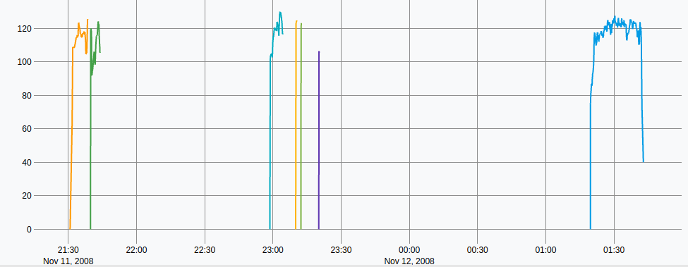
The upper code is not perfect: the first data point is 0 km/h, because the mapper window width is only one data point on the first data point of each split. (This could be fixed with STRICTMAPPER)

Data exploration: the speed is around 120 km/h. Not a big surprise on this road.

Up to the formula given, consumption is roughly 13 liter/100 km. There are around 80 km, so the total amount of fuel burned should be around 13×0.8 = 10.4 liters.

At this point, we have the distances $distances and the speed $speedKmh for each data point.

For each data point, we can apply the given formula to compute the number of liters burned between each tick.

For each tick, I will compute the amount of liters burned by the engine, then sum all these data. Just the way I did for the total distance, with bucketizer.sum.

// Its fuel consumption approximation is 8 (liters/100km) × (speed (km/h) / 80) +1.
// One liter of fuel releases 2392g of CO2.
// How much CO2 did the car released while driving on the Route 66?
$speedKmh MERGE 8.0 80.0 / * 1.0 +

// instantaneous consumption (liter/100km)
$distances MERGE * 100000.0 /

// current consumption (liter)
[ SWAP bucketizer.sum 0 0 1 ] BUCKETIZE // sum all values

'totalLiters' RENAME 

The output is a GTS named "totalLiters", with only one data point that contains the total amount of fuel burned on the Route 66: 10.05 liters. (=24kg of CO2)

The full code is available as a playable snapshot here. You can insert STOP where you want, or try to improve it!

And the winner is…

And thanks for the gifts ???

Learned a lot of things, enjoyed participating and now winning ? pic.twitter.com/LoqY2SBLTg

— Nicolas Steinmetz (@nsteinmetz) May 10, 2021

Pierre Papin

Electronics engineer, fond of computer science, embedded solution developer.