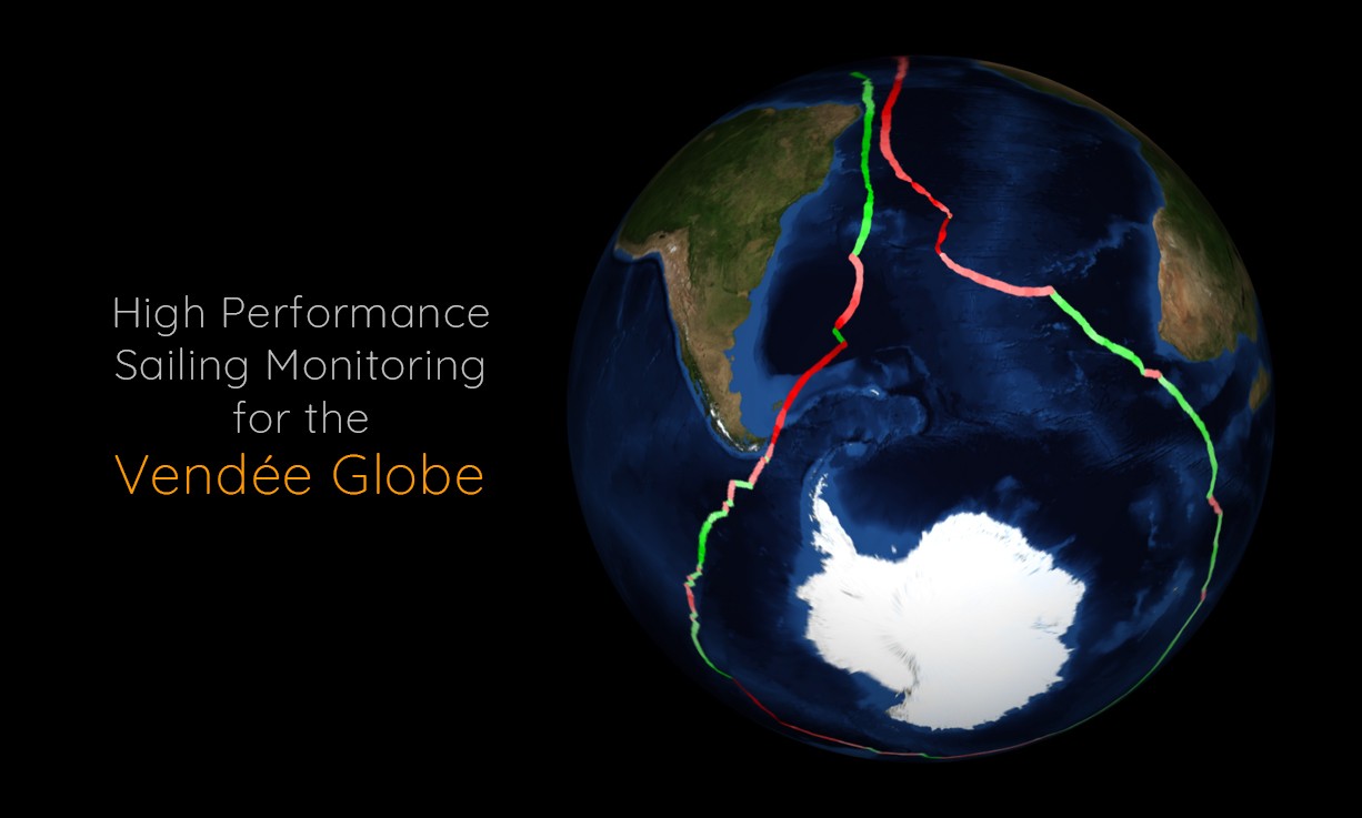
During the Vendée Globe 2020, Team Malizia monitored its yacht and gave access to this data. We jumped on the occasion to make some nice visualizations and analysis.
As I write these lines, the Vendée Globe 2020-2021 is still in progress and even if it's been more than 2 months since the start of the race, who will be the winner is still very much uncertain.
For those who are not familiar with the Vendée Globe, it's a non-stop, solo, and without assistance round the world yacht race. Sailors regard it as the technically, physically, and morally the toughest race.
The "without assistance" definition is quite complex though. It is indeed inadvisable, for security reasons, to forbid all communication between the sailor and her/his onshore team. On the other side, allowing free communication with the team could give too much assistance. That's why the Vendée Globe rules try to find the right balance. For instance, sailors can receive technical advice, medical advice, and weather forecasts in the form of offshore routing.
Only one team transmitted its data
What is of interest to us, are the rules concerning the transmission of data from the boat to the onshore team. The 4.3.3. Performance support section of the rules states that:
It is prohibited […] to send data from the boat to land which could be used to analyze and improve
Notice of race, Vendée Globe 2020-2021
performance except if they are made public instantaneously on reception.
It happens that only one team makes its data public: Team Malizia / Yacht Club de Monaco with their sailor Boris Herrmann. Team Malizia chose a Grafana dashboard to make data instantaneously available to the public. This provides a nice visualization of the data, but it is not straightforward to extract the data from it.
As SenX is not working or affiliated with Team Malizia, we had to find a way to retrieve the data, which we won't detail here. As you can expect, we stored the data in Warp 10 which allows us to easily manipulate the data.
For instance, here is a sample of the True Wind Speed (TWS) for an hour:

Visualization
The first thing we want to do is to explore the data with visualizations. We will only show the resulting images in this section, the scripts being too long.
It happens that a yacht is a perfect example of why Geo Time Series exist: the values of sensors change over time but are also dependent on the GPS coordinates.
Track and Point of Sail
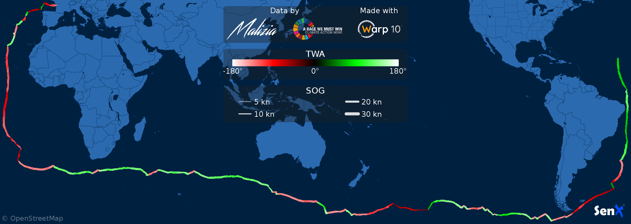
As the yacht sails over the ocean, wind conditions change as well as the boat speed. We want to visualize these changes, better understanding how the boat was helmed. The first two sensors we need are GPS latitude and longitude. We also need the True Wind Angle (TWA) which is the wind angle relative to the boat direction. Finally, we are interested in the speed which is called Speed Over Ground (SOG).
TWA is really important because it can give us information on the point of sail of the yacht, that is if it sails with the wind coming from port or starboard, but also upwind or downwind. These points of sail directly affect boat performance.
With this data and the Pstroke, PstrokeWeight, and Pline functions, it is quite simple to draw the track with SOG and TWA information. The background map is from OpenStreetMap and is modified with the Ptint and Pblend functions:
It is also possible to project a very similar image on a globe to better grasp the traveled distance.
Real Polar
Another very used visualization for racing yachts is polars. They summarize the performance of the boat in different wind conditions and help visualize VMG. However, they are theoretical performances, and sailors cannot be at "100% polar" during the whole race.
How to make nice data visualization and analysis of the monitoring of Team Malizia yacht during the #VendeeGlobe with real polar and point of sail track Share on XWe have the chance here to have the data for almost the whole race. So it is possible to plot the speed of the boat with respect to the TWA and TWS (True Wind Speed). The major flaw here is that we have only the SOG which is impacted by the current, nonetheless, it will give us a good idea of the performance of the boat in real conditions.
First, we take the median of the TWA, TWS, and SOG values every 10 seconds. This smooths the data, removing gusts of wind for instance. Then, once again, we use the Processing functions to draw a custom visualization:
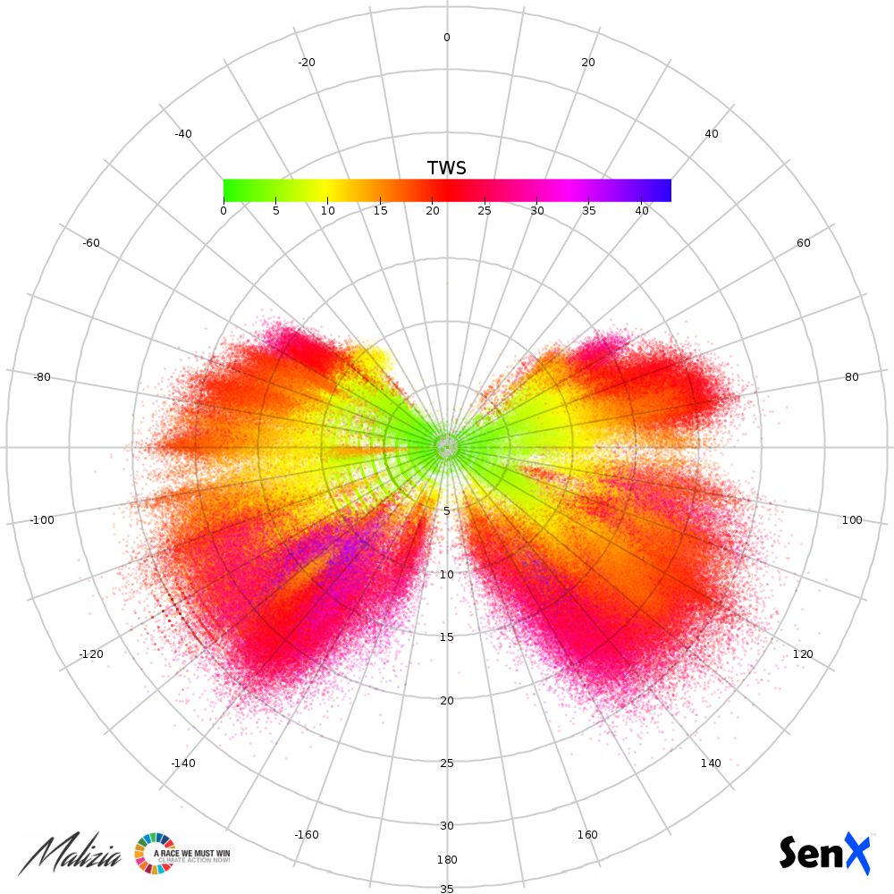
We're no expert at racing yachts, but it appears the best upwind VMG is around 10 kn and around 22 kn downwind.
Also, an interesting feature of this plot is that it seems symmetrical, but not quite so. It may be because the wind and condition were somewhat different between port and starboard or because of the currents. Finally, we also see that when there are strong winds, the speed is not that good, probably not to break anything. You can see that with the 2 purple spots at -140° and -125° between 10 and 15 knots.
Sea Temperature, CO2 and Salinity
On top of sensors for performance, Malizia is equipped with ocean sensors to measure water temperature, CO2 and, salinity. A visualization of these levels on the map has already been done, and a comment suggests there are relations between these values: cold water can store more CO2 and warm water evaporates more, leading to more salt in the water.
We can see if data corroborate this by simply drawing salinity and CO2 with respect to temperature. To avoid any problem with outliers, we draw the 5, 50, and 95-percentiles:

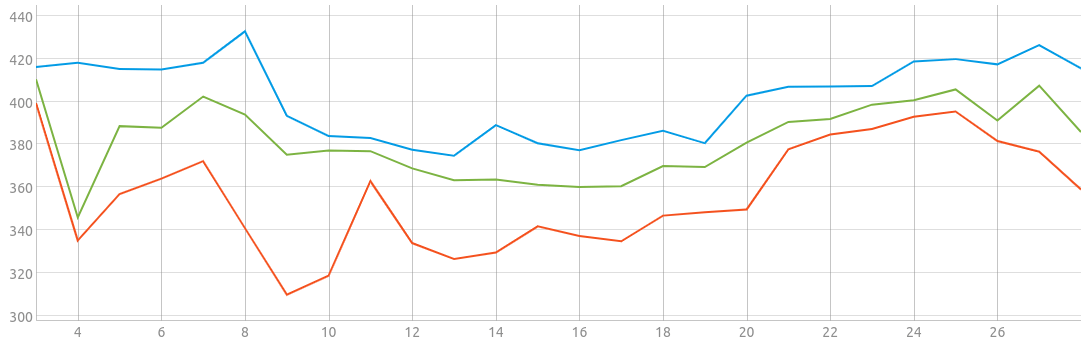
There is a clear relationship between temperature and salinity. The higher the temperature, the saltier the water is. This is true, except for temperatures of more than 26 °C, so that's not that simple. For CO2, there are probably other factors influencing its concentration, because it seems rather independent of the temperature.
Analysis
Until now, we focused on visualizing the data, which is great to have an overall view of the boat performance, and its sailing conditions. However, it is possible to detect and focus on peculiar moments, even in the middle of more than 2 months of data.
G-Forces
During the race, boats and sailors are subject to impressive shocks. Proofs are the video of the cracks Alex Thomson had to repair and Kevin Escoffier sinking.
There are G-force sensors on Malizia which can give us an idea of the number and power of these shocks. For instance, this short FLoWS script counted as many as 216245 g-force positive peaks!
vert = FETCH([token, 'com.team-malizia.ES.INS_VertAcc', {}, end, end - start])
mapper.peak = MACROMAPPER((mw) -> {
   return IFTE(
    AND(mw[7][1] > mw[7][0], mw[7][1] > mw[7][-1]),
    () -> { return [0, NaN, NaN, NaN, 1 ] },
    () -> { return [0, NaN, NaN, NaN, NULL()] }
  )})
return SIZE(MAP([vert, STRICTMAPPER(mapper.peak, 3, 3), 1, 1, 0])[0])
The force of each of these shocks is highly variable though. The most dangerous ones, obviously are the most powerful ones. We can sum vertical and horizontal g-force and find the highest values as follows
vert = FETCH([token, 'com.team-malizia.ES.INS_VertAcc', {}, end, end - start])
vert_abs = MAP([vert, mapper.abs(), 0, 0, 0])
vert_buck = BUCKETIZE([vert_abs, bucketizer.max(), end, m(1), 0])
horz = FETCH(['READ', 'com.team-malizia.ES.INS_HorAcc', {}, end, end - start])
horz_abs = MAP([horz, mapper.abs(), 0, 0, 0])
horz_buck = BUCKETIZE([horz_abs, bucketizer.max(), end, m(1), 0])
force = vert_buck[0] + horz_buck[0]force_big = MAP([force, mapper.ge(10), 0, 0, 0])
return TIMESPLIT(force_big, 1, 1, 'split')
This allows us to find 2 shocks of over 14 g and a lot of shocks on 10-11 November 2020. For the former, it's hard to tell if the data is correct or not, but for the latter, Boris Herrmann indeed encountered a rough sea during this period.

Loads
In the same way that g-forces gives an idea of the forces between the sea and the hull of the boat, we can study the forces the wind applies to the mast. Malizia is equipped with sensors measuring loads on the structures holding the mast. Simply looking at the sum of the forces on these structures (outriggers, runners, bobstay and J2), we can measure how much wind affected the boat:
loads = FETCH([token, '~com\.team-malizia\.(WTP_rename.outrigger.*|rig_.*_Runner|rig_bobstay_cal\.Load_Bobstay|rig_J2_cal\.Load_J2)', {}, end, end - start])
loads_buck = BUCKETIZE([loads, bucketizer.median(), end, m(10), 0])
loads_buck_sum = REDUCE([loads_buck, [], reducer.sum()])
loads_buck_small = MAP([loads_buck_sum, mapper.le(18.0), 0, 0, 0])
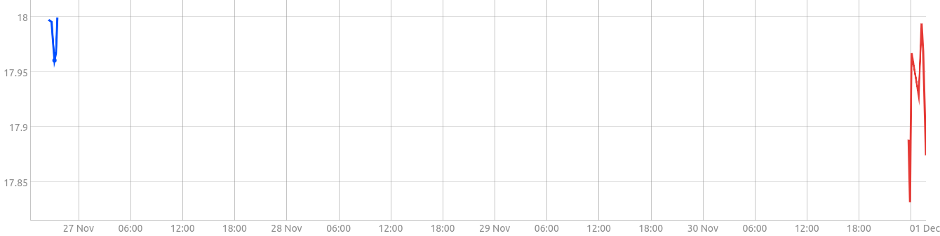
return TIMESPLIT(loads_buck_small, h(1), 4, 'split')Here we have the two moments when the total load was under 18t. The blue line is when Boris Herrmann went to the top of his mast to repair a hook and the red line is when he was searching for Kevin Escoffier. So using the only load, we can detect key moments in the race.
In the same manner, we can find total loads over 30t:
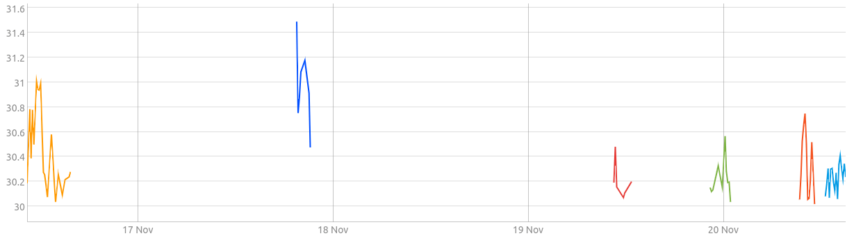
This result is more surprising because these high loads are only found between November 16 and 20, 2020. Has Boris Herrmann been more aggressive or has the weather condition been particular? We don't know.
Energy Generation and Number of Days
On a lighter note, on the already long list of sensors Team Malizia provides data from, there is the energy generation of the solar panels. As the energy generation depends on sun exposure, it is very easy to count the number of days since the beginning of the race:
end = NOW()
start = TOTIMESTAMP('2020-11-08T13:20:00z')
energy = FETCH(['READ', 'com.team-malizia.NRJ_Solar_cal.ISolar', {}, end, end - start])
energy_buck = BUCKETIZE([energy, bucketizer.median(), end, m(10), 0])
energy_buck_n0 = MAP([energy_buck, mapper.ge(0.15), 0, 0, 0])
return TIMESPLIT(energy_buck_n0, h(6), 5, 'day')
Which gives us:
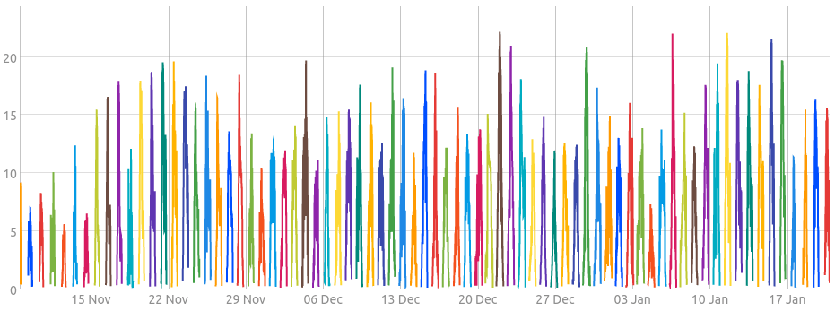
That makes 75 days. But between the time I write these lines, 20 January 2020, 22:00 GMT, and the start of the race, there are only 74 days! Sounds like Phileas Fogg, right? Anyway, sailors enjoy one more sunrise and sunset than us.
Takeaways
Ocean, wind, and boat interact in many ways during a race: the performance of a boat depends on the wind and sea conditions. A team wanting to increase the performance of its boat must have a deep understanding of its boat to get the best out of it without damaging it.
That's why yachts embark more and more sensors which can generate a fair amount of data. These data can be difficult to visualize and analyze without the right tools. Warp 10 is a suitable solution allowing blazing fast access to your data as well as providing more than 1000 functions to analyze it.
We, at SenX, are experts at data but not at racing yachts. In case you need someone to help you with the analysis of the data of your boat, we strongly encourage you to contact AIM45 which uses our solution and are experts at racing yachts.
Read more
Drawing Server Side - part 1
Review of DELL compatible batteries using Warp 10
Connect Power BI to Warp 10

WarpScript™ Doctor