How does a time series correlates with its past?

When working with a time series, one question that sometimes arises is whether it is similar to a past version of itself.

For this purpose, here comes the auto-correlation function (ACF). The ACF is a function of a lag τ. It is the correlation between the time series and itself when shifted back by τ. In other words, the greater the value of the ACF for lag τ, the more the time series correlates with itself when shifted back by τ. This is useful since for example, a high auto-correlation value means that the time series is seasonal.

This very interesting article – that I recommend to read – gives good examples of things you can do with the ACF.

However, since their data is stored in InfluxDB and that its query language is limited (it's not a complete programming language like WarpScript), their whole code is in Python. It introduces a processing overhead due to data conversion and serialization. If you are a user of Warp 10 and Python, you may already know that this pitfall can be mitigated. See for example our previous articles on the Py4J plugin for Warp 10 and WarpScript in Jupyter notebooks.

Moreover, the ACF can be directly computed in WarpScript. This is the subject of the following sections. We will give examples using this dataset.

One incentive of doing a bigger part of your processing with WarpScript is that it is well integrated with the ecosystem. For example, you can use the integration with Spark to parallelize your WarpScript.

Remember that you can reproduce the results on this article and play with this data in no time on the free Warp 10 sandbox.

Calculating the ACF in WarpScript

There are a multiple way to compute the ACF of a time series in WarpScript. The easiest is probably by using CORRELATE, which implements the correlation function.

CORRELATE takes 3 arguments:

1. The input time series (bucketized and without missing values)
2. A list of time series with which the correlation will be computed. For the ACF, we will provide a singleton list with a duplicate of the first argument
3. A list of lags for which the correlation will be computed

In our case, the result of CORRELATE will be a singleton list containing a GTS. The ticks of this GTS are the lags chosen by the 3rd argument, and its values are the associated ACF values.

For example, let us try it out on hourly temperature measurements in San Francisco:

// Fetching the data
[ 2012 ] TSELEMENTS-> ISO8601 'start' STORE
[ 2018 ] TSELEMENTS-> ISO8601 'stop' STORE
[ '<insert-your-token-here>' 'temperature' { 'city' 'San Francisco' } $start $stop ] FETCH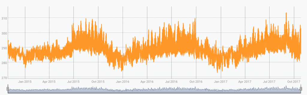

Now we compute the ACF:

// Ensure 1-hour buckets and interpolate missing values
[ SWAP bucketizer.mean 0 1 h 0 ] BUCKETIZE
INTERPOLATE
0 GET 'gts' STORE

// Compute ACF up to 1-year lag
$gts [ $gts ] [ 1 24 365 * <% h %> FOR ] CORRELATE

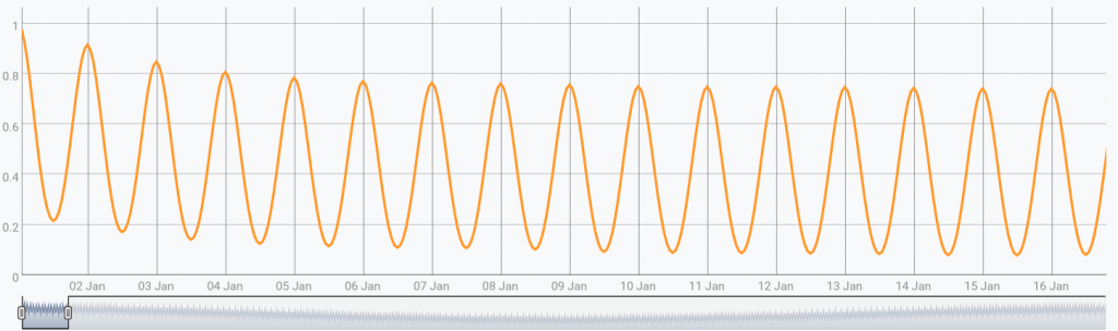
If we zoom in the result, we see that daily auto-correlation is obvious:

On the global picture, we can also notice a yearly auto-correlation:

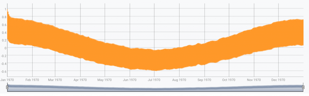
Note that ticks on the horizontal axis are expressed in terms of lags, so that for instance "02 Jan" reads "1-day lag", and "Mar 1970" reads "2-month lag".

The fast ACF in WarpScript

In the previous section, the computation of the ACF has complexity O(n²), which is prohibitive for most industrial (and bigger) datasets.

Hopefully, a fast approximation of the ACF can also be implemented using the fast fourier transform, that reduces the complexity to O(nlog(n)), according to the discrete case of the Wiener-Khinchin theorem.

Of course, WarpScript happens to have the FFT, and its inverse IFFT, ready off-the-shelf!

Let's modify the previous example for fast computation of the ACF:

// Compute the Fast Fourier Transform
$gts STANDARDIZE FFT
// To obtain the fast ACF, we compute the power spectrum and apply the Inverse Fast Fourier transform (Wiener-Khinchin theorem)
LIST-> DROP [ 're' 'im' NULL ] STORE
$re $re * $im $im * + $re $re - IFFT
// We shrink the result to the desired size (1 year), normalize using ACF(0) and rescale it to obtain interpretable results
24 365 * SHRINK DUP 0 ATINDEX 4 GET / 1 h TIMESCALE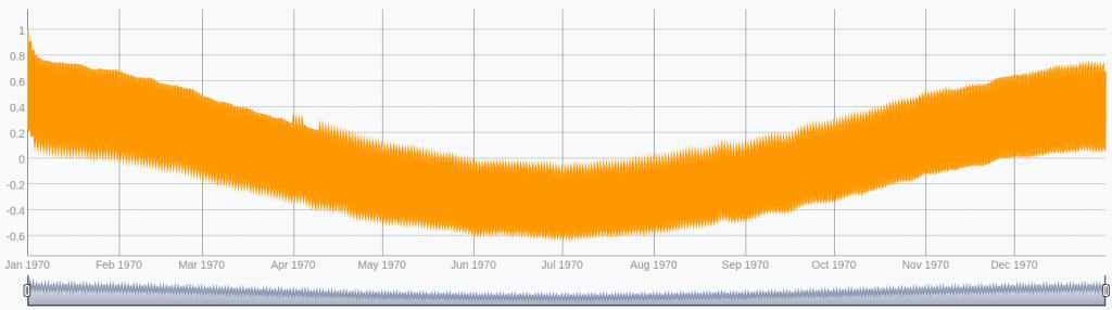

On the tested dataset, computing the ACF with the first WarpScript took about 30s. With the later WarpScript, it took only about 34ms, which is approximately 880 times faster.

Conclusion

In this article, we have presented the ACF, a function used to find out if a time series correlates with itself in the past. We showed how to implement it in WarpScript, with an exact calculation (but slow), and a fast one using the FFT (which accuracy is excellent despite being much faster).

Jean-Charles Vialatte

Machine Learning Engineer