Introduction
In WarpLib, prior to release 3.3.0, there were functions available for interpolation tasks. For example, INTERPOLATE fills empty time buckets with linear interpolation, and POLYFIT fits an interpolating polynomial to a series. These interpolations were supported on the time axis, meaning the estimation was based on timestamps.
With the release of Warp 10 version 3.3.0, new WarpScript functions were introduced to calculate multi-dimensional interpolation functions. Unlike previous functions that were timestamp-based, these new functions perform value-to-value interpolations.
New WarpScript Interpolation Functions
The following WarpScript functions have been introduced:
INTERPOLATOR.1D.LINEARINTERPOLATOR.1D.SPLINEINTERPOLATOR.1D.AKIMAINTERPOLATOR.2D.BICUBICINTERPOLATOR.3D.TRICUBICINTERPOLATOR.ND.MICROSPHEREINTERPOLATOR.ND.SMICROSPHERE
These functions return a callable function that estimates the values of points located between the sample points. The resulting function can be called using EVAL. If it is univariate, it can also be used as a mapper with MAP. If it is multivariate, it can also be used as a reducer with REDUCE.
Example Usage 1: 2D Bicubic Interpolation
Here’s an example demonstrating the usage of INTERPOLATOR.2D.BICUBIC. This function requires the estimates of sample points located on the knots of a 2D grid.
[ 10 40 100 190  ] 'xval' STORE
[ 10 50 180  ]  'yval' STORE
[ [ 50 0 255  ]
  [ 80 255 50 ]
  [ 100 0 30  ]
  [ 200 150 40  ] ]
'fval' STORE

$xval $yval $fval INTERPOLATOR.2D.BICUBIC
'interpolatingFunction' STORE
In this snippet, INTERPOLATOR.2D.BICUBIC takes three arguments. The first two, xval and yval, are the coordinates of the control points, and the third argument, fval, are the values of the function at these points.
That is, the control points and estimates are:
- 10, 10 -> 50
- 10, 50 -> 0
- 10, 180 -> 255
- … etc …
- 190, 180 -> 40
The resulting function interpolatingFunction can be called to estimate the value of a point within the range of the control points, which is x in (10, 190) and y in (10, 180). Outside of its scope, it will return a NaN value.
Visualizing the Interpolation
To illustrate this function, we can draw the control points:
// Initialize the image and the frame
200 200 '2D' PGraphics
255 Pbackground
1.01 PstrokeWeight

// Draw the circles and fill them
$xval
<%
  [ 'x' 'xi' ] STORE
  $yval
  <%
    [ 'y' 'yi' ] STORE
    $fval $xi GET $yi GET 'v' STORE
    $v Pfill
    0xFFFF0000 Pstroke
    $x $y 10 10  Pellipse
  %>
  T FOREACH
%>
T FOREACH

// Encode the image
Pencode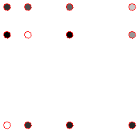
The red circles are drawn at the coordinates given by xval and yval. The grayscale filling the circles is defined by the values of fval.
Filling the Frame with Estimates
Now, we will fill the frame with estimates:
200 200 '2D' PGraphics
255 Pbackground
1.01 PstrokeWeight

// Interpolate all pixels (between black and white)
0 199
<%
  'x' STORE
  0 199 <%
    'y' STORE
    [ $x $y ] $interpolatingFunction EVAL 'color' STORE
    $color ISNaN <% 0x86FF0000 'color' STORE %> IFT // Out of range
    $color Pstroke
    $x $y Ppoint
  %>
  FOR
%>
FOR

// Encode the image
Pencode
In this image, the pixels have grayscale estimated values. The red pixels indicate those that are out of the scope of the interpolation function.
Example Usage 2: 3D Tricubic Interpolation
In this second example, we estimate an efficiency measure defined by the values of two pressure sensors and one temperature sensor. We use INTERPOLATOR.3D.TRICUBIC to create the interpolating function from a 3D grid of sample points.
[ 5 40 100 190 ] 'Pa' STORE
[ 10 50 180 ] 'Pb' STORE
[ -40 80 ] 'T' STORE

// Efficiency
[ [ [ 25.1 35 ]         // eg 25.1 is the efficiency for Pa = 5, Pb = 10, T = -40
    [ 18 32 ]
    [ 15 26 ] ]
  [ [ 125 135 ]
    [ 118 132 ]
    [ 115 126 ] ]
  [ [ 225 235 ]
    [ 218 232 ]
    [ 215 226 ] ]
  [ [ 325 335 ]
    [ 318 332 ]
    [ 315 326 ] ] ]
'E' STORE

$Pa $Pb $T $E INTERPOLATOR.3D.TRICUBIC
'interpolatingFunction' STORE
Now, given sensors producing values in GTS, we can derive the efficiency GTS.
// Generate synthetic data for the example
[
  100 @senx/rand/RANDOMWALK 7 2 0 2 RLOWESS
  NORMALIZE 185 * 5 +
  'pressure A' RENAME

  100 @senx/rand/RANDOMWALK 7 2 0 2 RLOWESS
  NORMALIZE 170 * 10 +
  'pressure B' RENAME

  100 @senx/rand/RANDOMWALK 7 2 0 2 RLOWESS
  NORMALIZE 120 * 40 -
  'temperature' RENAME
]
'gtsList' STORE

// Compute the estimate
[ $gtsList [] $interpolatingFunction ] REDUCE 0 GET
'Efficiency Estimates' RENAME
$gtsList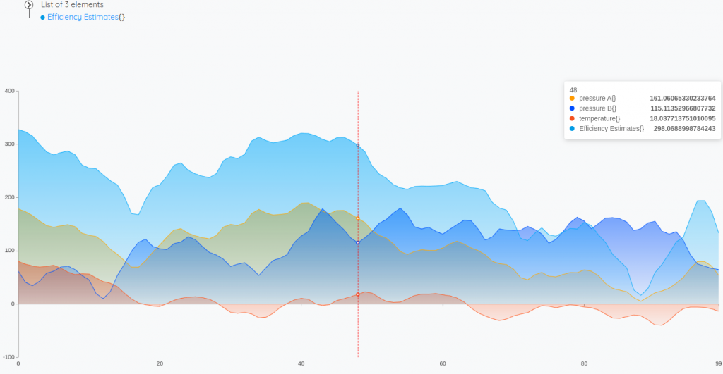
Conclusion
In this blog post, we presented the new multi-dimensional interpolation functions added in WarpLib with the release of Warp 10 version 3.3.0. These functions, prefixed with INTERPOLATOR.*, enable value-to-value interpolations across multiple dimensions. We demonstrated how these functions work through examples, including estimating values on a 2D grid and a practical use case with 3D sensor data.These new functions make it easier to handle value-to-value interpolation tasks in WarpLib.

Machine Learning Engineer